SFXC workshop 2025 • Pulsar processing
On this page
Introduction
Pulsar processing is special in the sense that
- the signal is dispersed and that
- the pulsar is “off” most of the time.
The dispersion is caused by the fact that the signal traverses the interstellar medium which is filled with free electrons at varying densities $n_e$. This does not only lead to multi-path propagation but, as such, the medium has a frequency dependent index of refraction which in turn leads to lower frequencies arriving later at the observer than higher frequencies. This time delay, $\Delta t$, is proportional to the total amount of electrons along the line of sight $dl$ – the dispersion measure or ${DM}=\int n_e\,dl$ – and it is proportional to the square of frequency:
$\frac{\Delta t}{\text{[ms]}} = 4.15 * \text{DM} * \left [\left (\frac{\nu_{\text{low}}}{[\text{GHz}]}\right )^{-2} - \left (\frac{\nu_{\text{high}}}{[\text{GHz}]}\right )^{-2}\right]$
Thus, in order to achieve the highest signal-to-noise possible, the data need to be de-dispersed at the correct dispersion measure and we can apply a technique called gating to only correlate the data when the pulsar is “on”. In this tutorial we will use SFXC to first generate filterbank format files (intensities as a function of time and frequency) from the single dish data. We will take a quick peak at what a pulsar looks like in the data and we’ll use SFXC’s capabilities of creating coherently dedispersed, full polarisation filterbanks to create a folded full polarisation pulse profile of the pulsar B1933+16.
Eventually, we will use standard pulsar tools to generate a so-called “polyco” file, a file that contains the polynomial coefficients used to predict the time of arrival (TOA) of individual pulses. It is these TOAs that the correlator needs to extract only the chunks of data when the pulsar is “on”. We will generate gated output files and also take a look at pulsar binning – this is when we do not use only one on-off gate but instead place several bins across the pulse profile. This can either be used to boost the S/N of correlated pulsar data even further by weighting the data according to the brightness of the pulsar per bin (Deller 2009, Keimpema et al. 2015) or one can, e.g., perform phase-resolved pulsar scintillometry (Pen et al. 2014).
Data download
In this tutorial we’ll use data from a recent pulsar observations. Ideally, you’ll create a new directory somewhere and download all files there. The files we’ll download are as follows:
aux-config.tar          : contains a few control files, vex files and polycos
pr359a_ef+o8+ur_10s.tar : (~9GB) the raw baseband data from Ef, Ur, O8; 10s each
psrsoft.simg            : (~6GB) singularity image containing the pulsar tools we need
sfxc-coherent.simg      : (~400MB) SFXC that supports coherent dedispersion
On the JIVE cluster your will find those data at /data/pr359a. Ideally leave that
baseband data and the images where they are but copy aux-config.tar to your directory of
choosing and untar it there. Modify the paths in the ctrl files to point at where the data
are and set the output and delay directories to your directory of choosing.
In caes you’d like to run things on your local laptop, proceed as follows:
mkdir /path/to/your/dir
cd !$
files='aux-config.tar pr359a_ef+o8+ur_10s.tar psrsoft.simg sfxc-coherent.simg'
for f in $files;do wget https://archive.jive.nl/sfxc-workshop/pr359a/$f;done
tar xf aux-config.tar && rm -rf aux-config.tar
tar xf pr359a_ef+o8+ur_10s.tar && rm -rf pr359a_ef+o8+ur_10s.tar

# there are a few places in the control file where we need to know in which
# directory things are -- let's fix that
this_dir=`pwd`
sed -i -e "s,/<<path/to>>,${this_dir},g" *ctrl
Producing filterbank format output + run PSR tools
Let’s generate a filterbank file from the baseband data of one of the stations in our observations. We chose to use the data from Effelsberg as it is the most sensitive dish in the array.
The aim of this exercise is to a) introduce the pulsar-related capabilities of SFXC and b) show some basics of pulsar analysis software.
Prepare the vex file
The vex file as it was generated using sched (or pysched) does not yet contain all the
info required by the correlator. E.g., it’s missing the CLOCKS section as well as the EOP
section. This can be fixed by running
# if you do run the below, please note that I delieberately messed up the suffix of the
# output file to avoid the actual vix file form being overwritten.
prepare_vex.py pr359a.vex pr359a.vixx
This utility is shipped with SFXC. The generated vix file contains the correct sections
but the CLOCKS will all be zero. To get the clock delays right one would now perform
clock searching. Here we have already fixed the clocks for the stations relevant for this tutorial:
Ef, Ur, O8 in the provided vix file.
Prepare the ctrl file
As a first step we’ll create a 10s-filterbank as outlined below:
{
    "number_channels": 8,           # number of channels per subband
    "cross_polarize": false,        # only correlate LL and RR
    "integr_time": 1.024,           # in seconds needs to be an integer multiple of:
    "sub_integr_time": 256.0,       # sub_integr_time (in us); cannot be less than the time equivalent of (depends on the sampling rate of course):
    "fft_size_correlation": 128,    # number of samples per FFT;
    "start": "2025y244d17h31m10s",
    "stop": "2025y244d17h31m20s",
    "filterbank": true,             # generate output that can be converted to filterbank
    "output_file": "file:///path/to/pr359a_ef_no0001_b1933_10s.cor",
    "delay_directory": "file:///path/to/delay-tables/",
    "data_sources": {
        "Ef": [
            "file:///path/to/pr359a_ef_no0001"
        ]
    },
    "stations": [
        "Ef"
    ],
    "channels": [
        "CH01",
        "CH02",
        "CH03",
        "CH04",
        "CH05",
        "CH06",
        "CH07",
        "CH08",
        "CH09",
        "CH10",
        "CH11",
        "CH12",
        "CH13",
        "CH14",
        "CH15",
        "CH16"
    ],
    "exper_name": "pr359a",
    "normalize": false,
    "window_function": "NONE",
    "message_level": 1
}
Run the correlator and convert the output to filterbank
mpirun -n 22 sfxc pr359a_ef_no0001_b1933.ctrl pr359a.vix

# if using the singularity image:
mpirun -n 22 singularity run /path/to/sfxc-coherent.simg sfxc pr359a_ef_no0001_b1933.ctrl pr359a.vix

# or in the cluster using the image
srun --mpi pmix -n 2 singularity run /path/to/sfxc-coherent.simg sfxc pr359a_ef_no0001_b1933.ctrl pr359a.vix
TIP: In case the above gives you an error about not enough cores present, you may need to add
--oversubscribe. On a machine where you have enough cores and still get an error about not enough cores, try adding--use-hwthread-cpus.
The output file will be at /path/to/pr359a_ef_no0001_b1933_10s.cor_Ef – note the suffix
Ef since this is for station Effelsberg. Now we’ll convert this to filterbank format as
regular pulsar software cannot handle the output format of SFXC.
cor2filterbank.py pr359a.vix pr359a_ef_no0001_b1933_10s.cor_Ef pr359a_ef_no0001_b1933_10s.cor_Ef.fil

# if using the singularity image either execute like this:
singularity run /path/to/sfxc-coherent.simg /usr/local/src/sfxc/frb_runjob/cor2filterbank.py pr359a.vix pr359a_ef_no0001_b1933_10s.cor_Ef pr359a_ef_no0001_b1933_10s.cor_Ef.fil

# or enter into an 'interactive' session
singularity shell -e /path/to/sfxc-coherent.simg

# and run like so:
/usr/local/src/sfxc/frb_runjob/cor2filterbank.py pr359a.vix pr359a_ef_no0001_b1933_10s.cor_Ef pr359a_ef_no0001_b1933_10s.cor_Ef.fil
cor2filterbank.py has a bunch of different options. Above we’re running it at defaults,
generating a Stokes I filterbank. Options are:
cor2filterbank.py --help
Usage: Usage : cor2filterbank.py [OPTIONS] <vex file> <cor file 1> ... <cor file N> <output_file>

Options:
  -h, --help            show this help message and exit
  -i IFS, --ifs=IFS     Range of sub-bands to correlate, format first:last.
                        For example -i 0:3 will write the first 4 sub-bands.
  -s SETUP_STATION, --setup-station=SETUP_STATION
                        Define setup station, the frequency setup of this
                        station is used in the conversion. The default is to
                        use the first station in the vexfile
  -b, --bandpass        Apply bandpass
  -z, --zerodm          Apply zerodm subtraction
  -d, --decimate-freq   Compensate for zeropadding by removing the odd
                        numbered frequency points, default=no
  -p POL, --pol=POL     Which polarization to use: R, L, I (=R+L), or F(=R,
                        Re(RL), Im(RL), L), default=I
Take a look at what’s in the filterbank
For the below we will work in the singularity image that contains all of the pulsar software tools that we need. It can be retrieved from here. Enter the image like so to run things interactively
singularity shell -e /path/to/psrsoft.simg
Now we can plot what’s in the filterbank with waterfaller.py that comes with the PRESTO
package. Here we’re using a slightly modified version that has some functionality added
to it, such as flagging channels and setting the dynamic range (can be found on Franz’
github). The outcome should look something like
Figure 1.
waterfaller.py --show-ts --show-spec -T 1.25 -t 1.2 --killchans 0-16,31,46-47,62-63 \
  pr359a_ef_no0001_b1933_10s.cor_Ef.fil --full_info --colour-map viridis \
  --vmin -1 --vmax 1
Tipp: In case no plots are being shown with the command above, you may need to set the environement variable
$DISPLAY. Before starting the image as shown above, check what the variable is set to in your terminal viaecho $DISPLAYOnce you’re in the image, you need to set$DISPLAYto whatever the outcome is of the above by runningexport DISPLAY=<output from above>
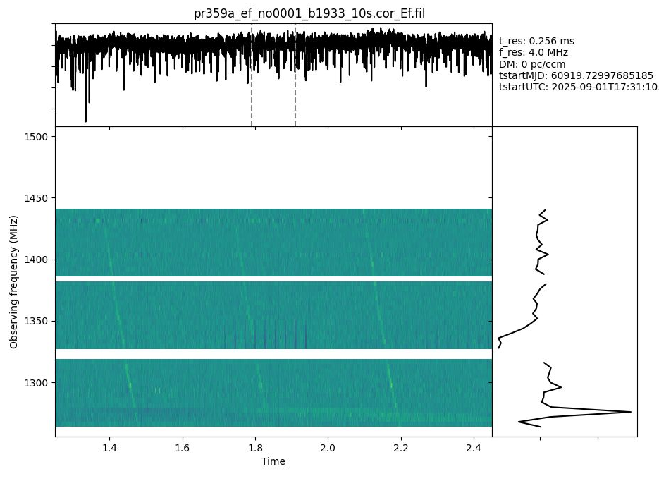
Figure 1 - Dynamic spectrum (main panel), frequency-collapses
time series (top panel) and time-averaged spectrum (right panel) as generated with
PRESTO’s waterfaller.py. Here we flagged the worst RFI, visible as white horizontal “lines”. One can
cleary see the quadratic sweep of the pulses, as well as more RFI. The pulses do not yet
pop out in the time series as they are still dispersed.
We can now apply incoherent dedispersion as it is provided by waterfaller.py via the
flag -d <DM> to get Figure 2
waterfaller.py --show-ts --show-spec -T 1.25 -t 1.2 --killchans 0-16,31,46-47,62-63 \
  pr359a_ef_no0001_b1933_10s.cor_Ef.fil --full_info --colour-map viridis \
  --vmin -1 --vmax 1 -d 158.52
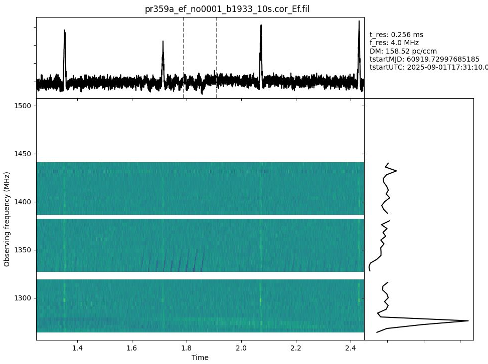
Figure 2 - Same as Figure 1 but with incoherent dedispersion applied.
And we can even zoom in on one pulse – see Figure 3. What you will see is that things do not align perfectly in frequency. This is caused by residual dispersion smearing; residual in the sense that not all the dispersion has been taken out, in particular that within a channel. We chose quite a crude channelisation just to show this effect. The amount of residual smearing $\delta \tau$ per bandwidth $BW$ at a certain central frequency $\nu$ is approximated as
$\frac{\delta \tau}{\mu s} = 8.3 * \frac{\text{BW}}{[\text{MHz}]} * \text{DM} * \left (\frac{\nu}{[\text{GHz}]}\right )^{-3}$
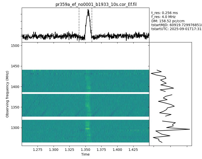
Figure 3 - Zoom in on a single pulse with incoherent dedispersion applied. The pulse does not appear “straight” in the dynamic spectrum because of residual dispersion smearing: we chose quite a crude frequency resolution leading to some dispersive delay being present within a channel.
Create full polarisation filterbank, fold and plot it
Here we have chosen a fairly bright pulsar for which we can see individual pulses in the Effelsberg data. If we were to run the above correlations on the Urumqi or Onsala data, we would not see individual pulses – try it out! However, if we were to fold the Ur or O8 data, we would very much see the pulsar in the “folded” data, i.e. data where we chop the data into chunks of the same length as the pulse period and add up the chunks. This will beat the noise down and have the signal appear. In many pulsar science applications, people are interested in that very folded profile, moreover in the polarisation characteristic. So let’s create a full polarisation folded profile of a pulsar.
{
    "number_channels": 128,            # <--- note we use more channels now to better compensate for residual smearing
    "fft_size_correlation": 128,
    "cross_polarize": true,            # <--- full Polarisation
    "integr_time": 1.024,
    "sub_integr_time": 256.0,
    "start": "2025y244d17h31m10s",
    "stop": "2025y244d17h31m20s",
    "output_file": "file:///path/to/pr359a_ef_no0001_b1933_10s_fullPol.cor", # <--- change output file name to not get confused later
}
# ---- everything else stays the same
- run the correlator
mpirun -n 12 --oversubscribe sfxc pr359a_ef_no0001_b1933_10s_fullPol.ctrl pr359a.vix
- convert the output with cor2filterbank but set the correct flags (
-p F)
cor2filterbank.py pr359a.vix pr359a_ef_no0001_b1933_10s_fullPol.cor_Ef pr359a_ef_no0001_b1933_60s_fullPol.cor_Ef.fil -p F
- create a “par” file (contains pulsar parameters like period, period derivative,
dispersion measure) with
psrcat:
# inside psrsoft.simg
psrcat -e B1933+16 > B1933+16.par
- run dspsr on the full polarisation filterbank file with the par-file that we just created:
dspsr -E B1933+16.par -L 1 -A -k effelsberg -d4 \
  pr359a_ef_no0001_b1933_10s_fullPol.cor_Ef.fil \
  -O pr359a_ef_no0001_b1933_10s_fullPol.cor_Ef.fil
#### Flags set here are:
# -E <par file>    : par file to use
# -L <seconds>     : number of seconds per "sub-integration"
# -A               : create a single output file (otherwise there will be one per "sub-integration" of 1s length
# -d <pol-product> : what polarisation product to create; the 4 means full pol
# -O               : output file base_name; .ar will be appended automatically
- flag the bad channels interactively (press ‘h’ to get instructions on the terminal)
# in psrsoft.simg
psrzap pr359a_ef_no0001_b1933_10s_fullPol.cor_Ef.fil.ar

# Two overlapping pgplot windows will op up: one with three panels
# showing:
#   - the time series
#   - one showing pulse phase vs. frequncy, and
#   - one showing pulse phase vs. time
# The second window is where you can flag sections in both time and frequency
#
# When you press 'h', the help should show the below
pzrzap interactive commands

Mouse:
  Left-click selects the start of a range
    then left-click again to zoom, or right-click (or 'X') to zap.
  Right-click (or 'X') zaps current cursor location.
  Middle-click (or 'D') updates the diagnostic plots.
Keyboard:
  h  Show this help
  f  Use frequency select mode
  t  Use time select mode
  b  Use time/freq select mode
  d  Update diagnostic plots
  v  Switch plot between variance and mean
  l  Toggle logscale
  m  Toggle method
  p  Switch to next polarization
  B  Toggle variable baseline removal
  u  Undo last zap command
  r  Reset zoom and update dynamic spectrum
  s  Save zapped version as (filename).zap
  P  Print equivalent paz command
  w  Generate PSRSH script
  Q  Save file then exit
  q  Exit program
- When you’re done flagging, write out the flagged file and exit via ‘Q’ (new file will
have suffix
zapinstead ofar. - Now let’s plot the folded full polarisation profile (should look like Figure 4.
psrplot -D /XWIN pr359a_ef_no0001_b1933_10s_fullPol.cor_Ef.fil.zap \
        -j tscrunch,dedisperse,fscrunch \   # summing up in time and frequency
        -p Scyl \                           # request full pol plot
        -c 'x:unit=ms' \                    # set the unit of the x-axis to 'ms'
        -c 'x:bin=650:900'                  # zoom in on phase bins 650-900
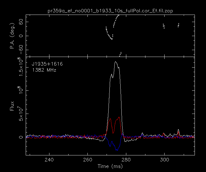
Figure 4 - Full polarisation profile of B1933+16, zoomed in on the pulse profile. The top panel shows the polarisation position angle swing while in the bottom panel the red and blue lines show the linear and circular polarisation intensity, respectively. The white line is the total intensity.
Generate coherently dedispersed filterbank with SFXC
Of course we can try and compensate for the residual smearing by increasing the number of frequency channels in the fitlerbanks as we have done above in the full polarisation examples. However, this will come at the cost of time resolution which in the case of a millisecond pulsar (or and FRB) will disable us to look for fine structure. Therefore we can use coherent dedispersion which removes any residual dispersion smearing also within a channel.
- prep the control file:
{
    "number_channels": 8,           # <--- we go back to the crude channelisation
    "cross_polarize": false,        # <--- turn off full polarisation
    "integr_time": 1.024,
    "sub_integr_time": 256.0,
    "fft_size_correlation": 128,
    "start": "2025y244d17h31m10s",
    "stop": "2025y244d17h31m20s",
    "output_file": "file:///path/to/pr359a_ef_no0001_b1933_10s_coher+incoher.cor",
    "filterbank": true,
    "pulsars": {                    # <--- here we switch on the "pulsar" mode which requires extra input
        "B1933+16_D": {             # <--- the source name has to match what's in the vex file
            "polyco_file": "file:///<<path/to>>/b1933.polyco",  # <--- contains the DM of the pulsar (amongst other things that we will need later)
            "no_intra_channel_dedispersion": false,     # <--- if set to true, the dispersion delay between subbands (IFs) will not be corrected for
            "coherent_dedispersion": true
        }
    },
### everything else stays the same
- we require a so-called polyco file which contains info about the pulsar; most important here the DM and the rotation frequency detailed info:
cat b1933.polyco
# name     date        UTC        MJD                         DM          DopplerShift  fit_rms
1935+1616  31-Aug-25   93000.00   60918.39583333330           158.521055  0.496         -8.844

#   reference phase     rotation frequency  observatory  data_span  n_coefficients  observing_frequency
   3488444629.211404    2.787546496219      coe          300        3               1400.000
#  Coefficent-1            Coefficient-2            Coefficient-3
  0.00000000000000000e-10 -0.00000000000000000e-02 -0.00000000000000000e-08
- run the correlator (with coherent dedispersion turned on, you’ll need a fair bit of memory)
mpirun -n 22 --oversubscribe sfxc pr359a_ef_no0001_b1933_10s_coher+incoher.ctrl pr359a.vix
- convert to filterbank
cor2filterbank.py pr359a.vix pr359a_ef_no0001_b1933_10s_coher+incoher.cor_Ef pr359a_ef_no0001_b1933_10s_coher+incoher.cor_Ef.fil
- plot again with waterfaller.py
waterfaller.py --show-ts --show-spec -T 1.25 -t 0.2 --full_info --colour-map viridis --killchans 0-18,30-32,44-47,57-63 --vmin -1 --vmax 1 pr359a_ef_no0001_b1933_10s_coher+incoher.cor_Ef.fil
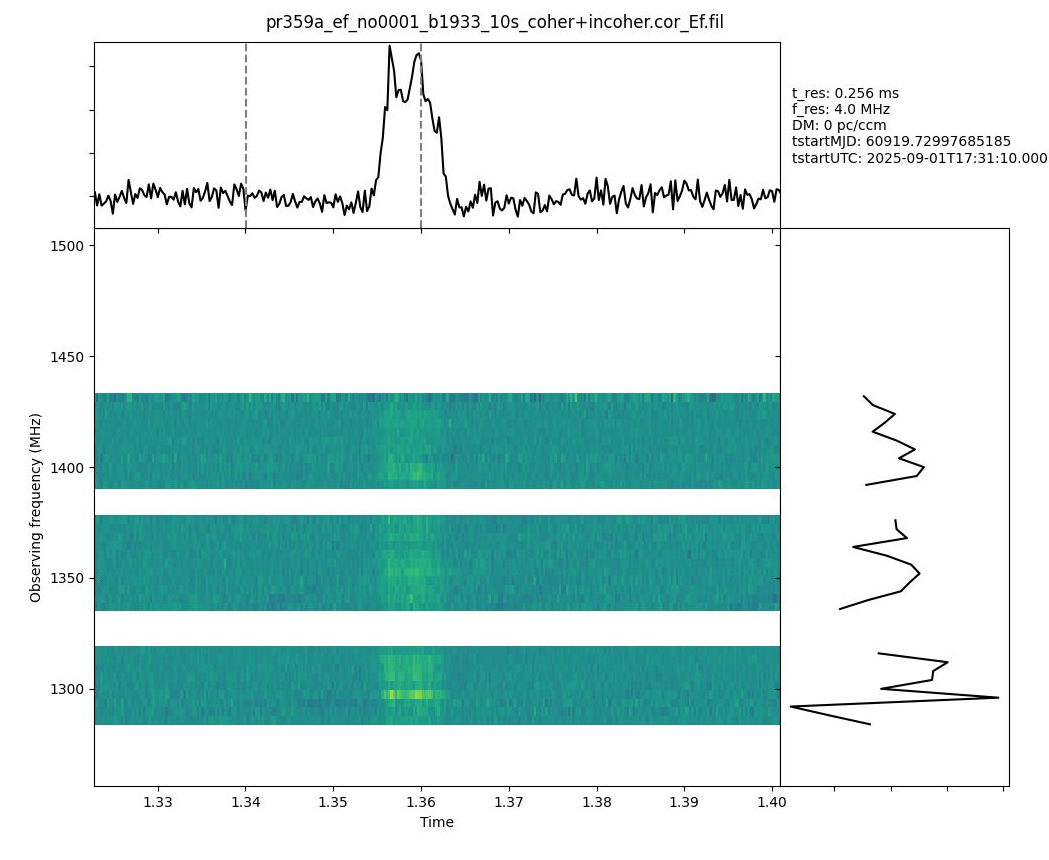
Figure 5 - Single burst coherently dedispersed. Substructure becomes evident now (compare to Figure 3).
Pulsar Gating
Now that we know what’s in the data and how folding works, let’s try pulsar
gating/binning. Here we accumulate only the data that contain a pulse to boost S/N. For
the correlator to be able to do so, it needs to “know” the TOAs of each pulse. This info
is provided by the polyco file which can be generated with tempo2 given a pulsar
parameter file.
Create polyco for gating.
We generated the par file above for folding. We can reuse it here to create a polyco that contains everything we need:
# from inside the singularity container psrsoft.simg we run
tempo2 -f B1933+16.par -polyco "60918 60920 300 12 8 coe 1400.0" -tempo1

# we are asking for coefficients between MJDs 60918 60920, we'd like a new set of
# coefficients avery 300 minutes, we're asking for a 12th order polynomial at a
# maximum hour angle of 8h; the TOAs should be for the center of Earth (coe) at a
# central frequency of 1400.0 MHz. Last but not least the output should be in
# tempo1 format.
# We will get 3 output files but we're only interested in polyco_new.dat. Let's rename it:
mv polyco_new.dat b1933-full.polyco
Prepare the ctrl file
The control file for the gating is similar to the one for coherent dedispersion in the sense that it needs the ‘pulsar’ section. Here we now change the output back to ‘regular’ output format (i.e. not ‘filterbank’) and be turn on pulsar binning. In addition, since we are not correlating in proper sense, we also add in where to find the data from Urumqi and Onsala:
{
    "number_channels": 128,
    "cross_polarize": false,
    "integr_time": 1.024,
    "start": "2025y244d17h31m10s",
    "stop": "2025y244d17h31m20s",
    "output_file": "file:///path/to/pr359a_ef-ur-o8_no0001_b1933_10s_fullPhase.cor",
    "filterbank": false,       # <-- for gating we need "regular" output files
    "pulsar_binning": true,    # <-- NEW PARAMETER: we turn on pulsar binning
    "pulsars": {
        "B1933+16_D": {
            "polyco_file": "file:///path/to/b1933-full.polyco",
            "coherent_dedispersion": false,   # we go for incoherent dedispersion to speed up the correlation;
            "nbins": 50,  # the number of phase-bins across the pulse period
            "interval": [
              0,          # we do the full phase range at first and refine later
              1
            ]
        }
    },
    "delay_directory": "file:///path/to/",
    "data_sources": {
        "Ef": [
            "file:///path/to/pr359a_ef_no0001"
        ],
        "Ur": [
            "file:///path/to/pr359a_ur_no0001"
        ],
        "O8": [
            "file:///path/to/pr359a_o8_no0001"
        ]
    },
    "stations": [
        "Ef",
        "Ur",
        "O8"
    ],
    "channels": [
        "CH01",
        "CH02",
        "CH03",
        "CH04",
        "CH05",
        "CH06",
        "CH07",
        "CH08",
        "CH09",
        "CH10",
        "CH11",
        "CH12",
        "CH13",
        "CH14",
        "CH15",
        "CH16"
    ],
    "exper_name": "pr359a",
    "normalize": false,
    "window_function": "NONE",
    "message_level": 1
}
- run the correlator
This will generate 51 output files with suffix .binXY, one fore each bin plus bin0
containing the “offpulse” data, i.e. that which is outside the interval. We can plot the
“pulse profile” with the script profile.py which is shipped with singularity image
sfxc-coherent.simg.
- plot the outcome form inside the container
sfxc-coherent.simg
/usr/local/src/sfxc/sfxc/utils/profile.py pr359a.vix pr359a_ef-ur-o8_no0001_b1933_10s_fullPhase.cor 50 Ef
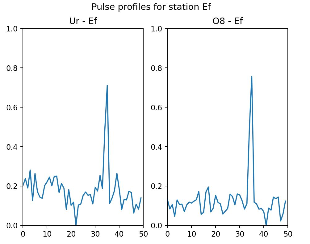
Figure 6 - Pulse “profiles” on the Ef-Ur and Ef-O8
baselines. The pulse period (~358.7ms) is broken up into 50 time bins (~7.2ms each) based on the
polynomial coefficients in ‘b1933-full.polyco’ as generated with tempo2. Each “set” of
data (10 seconds of data / 358.7ms pulse period = 28 chunks per bin) is
correlated individually and eventually summed up. The bin that contains the pulse clearly sticks out. In a way,
this is a “folded” pulsar profile at very crude time resolution.
We clearly detected the pulse in one of the bins. We can now refine the pulse interval to really get an “on-gate” – in our case we’ll go directly into binning to resolve the pulse profile:
- refine the gates, i.e. change the interval from [0,1] to [0.65, 0.75]
I.e., in the control file we’ll have the following
    "output_file": "file:///path/to/pr359a_ef-ur-o8_no0001_b1933_10s.cor", # change output name
    "filterbank": false,
    "pulsar_binning": true,
    "pulsars": {
        "B1933+16_D": {
            "polyco_file": "file:///path/to/b1933-full.polyco",
            "coherent_dedispersion": false,
            "nbins": 50,
            "interval": [
              0.65,          # zoom in on this phase range
              0.75
            ]
        }
    },
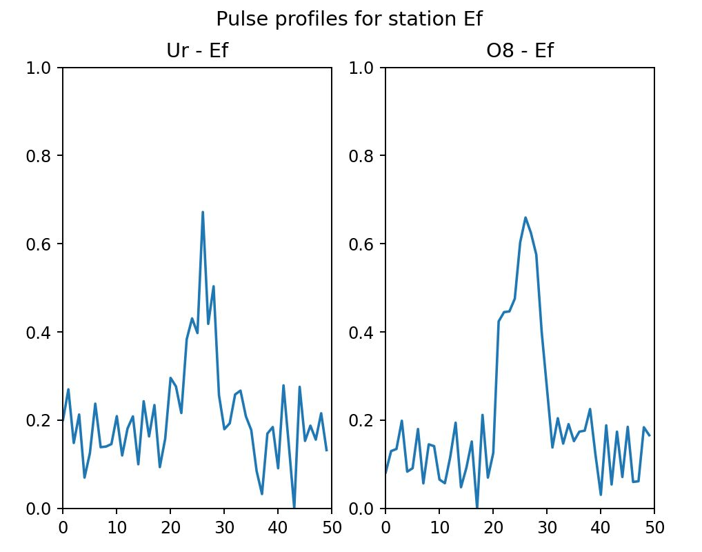
Figure 7 - Same as Figure 6 but zoomed in on the pulse phase range 0.65-0.75. Now the substructure also becomes available here.
At this point one would refine the interval even more to have only “on-bins”. As in
regular observations, the following steps are then to run tconvert and j2ms2 to create
fitsidi files that can then loaded into your favourite data reduction and calibration tool.
References
1. Deller, A. T., “Precision VLBI astrometry: Instrumentation, algorithms and pulsar parallax determination”, PhD Thesis, (2011). ADS: 2009PhDT…….195D
2. Keimpema, A., et al., “The SFXC software correlator for very long baseline interferometry: algorithms and implementation”, Experimental Astronomy, 39(2), 259–279 (2015). DOI: 10.1007/s10686-015-9462-z
3. Pen, U.-L., et al., “50 picoarcsec astrometry of pulsar emission”, MNRAS, 440, L36-L40 (2014). DOI: 10.1093/mnrasl/slu010
Content built by Franz Kirsten.
Built with ♥ — Markdown + HTML + CSS + Prism.js + a bit of AI + Jack Radcliffe (2025)